Many populations of astronomical objects follow power-law distributions in their proprties, also known as Pareto distributions to pretty much everyone else in the statistical world. Of note the masses of stars produced by the star formation process follows an initial mass function (IMF). When first calculated, the functional form of the IMF appears to follow a power-law distribution, though subsequent work has started to argue about whether this is actually the case. A reason for this debate is that physical processes, notably turbulence, can easily produce a log-normal distribution and it is difficult to distinguish between these two cases in the data. Lately, it appears that turbulence produces the log-normal and then gravity amplifies the positive wing of the log-normal to create a power-law. This leads to the truly awesome power-law-log-normal distributions which are finally getting some attention in astronomy (see Basu et al., 2015, Brunt et al., 2015).

With that preamble aside, a major goal is to estimate the parameters of a power-law distribution given observed data. Practically, we will be measuring the mass distributions of molecular clouds in a survey region. The mass distribution (represented as the differential number of clouds per unit mass interval) can then be represented as probability density function:

where $N_{\mathrm{tot}}$ is the total number of clouds in the system. The constant $\beta$ is a normalization constant and $\alpha$ is called the index. I like to define it to have no sign (because negative numbers are a thing), but many authors prefer to define it as positive number and include a negative sign in the formula. For the classic Salpeter IMF (a journal article with nearly 5000 citations), $\alpha=-2.35$. For GMCs, the index has been shown to vary in Rosolowsky 2005 between $\alpha = -2.5$ to $\alpha = -1.5$ depending on the system under study. We aim to measure this index. Furthermore, there is some evidence that there is a maximum mass for the distribution in some systems. We aim to calculate that mass:

Thus, we have a three parameter system: $\alpha, \beta$ and $M_{\mathrm{max}}$ that we are trying to determine from the data. We can do this a few different ways. The usual approach is to empirically estimate $dN/dM$ by calculating a discrete approximation $\Delta N/\Delta M$ where we count the number of clouds in some mass interval, say $3\times 10^5 M_{\odot} < M < 4\times 10^{5}M_{\odot}$. If there are, say, 20 clouds in this interval, then $\Delta N / \Delta M = 20 / 10^5 M_{\odot}$. Note that this means that $dN/dM$ has units of inverse mass and is intended to be integrated over. This is a fine approach, but it is biased in cases where there are a few points per mass bin and when the observational errors can move objects from one bin to the other. In the previous example, if the mass error is also $10^5 M_{\odot}$ then the cloud might appear in different bins in different observations.

To alleviate these issues, we focus on the cumulative mass function ($N(>M)$), or in statistics language the complementary cumulative distribution function (denoted cCDF). This is defined as

where the latter expression is the power-law case. In the case of a truncated power-law it is useful to express things in terms of the mass of the maximum cloud and the number of clouds near that mass $N_{\mathrm{max}}$:

This largely sets up the formalism. There are a few subtleties to deal with regarding observational errors and completeness limits, but this should get us started. We want to use python for this analysis, but like all things in python, there’s a package for it. To install the package, use the python package installer pip. From the Linux command line, type

pip install powerlaw
pip install mpmath

This will install two packages powerlaw and mpmath. The latter is needed for some of the calculations we may do later. The best documentation of the powerlaw package is in this article. To fit a power law to some data, it must be in the form of a numpy array. The classic analysis in GMCs is the mass distribution, so let’s look at the distribution of luminous masses derived from the $X_{\mathrm{CO}}$ factor.

import powerlaw
from astropy.table import Table
t = Table.read('mycatalog.fits')  # load into an astropy table
mass = t['MASS_EXTRAP'].data      # Pull out the mass variable into a numpy array.
myfit = powerlaw.Fit(data)

This loads the data and does the fit for you. Pretty cool! You can go ahead an look at the data:

myfit.plot_ccdf()

You can also check out the fitted index:

print(myfit.alpha)

You can also fit two different forms of the distribution. To do this, we activated the distribution_compare function.

R, p = myfit.distribution_compare('power_law','truncated_power_law`)

and this compares the two different distributions: an ordinary power law and a truncated version. Note that this package uses the definitions of Clauset et al. (2007) where the truncated power law has a form

Two things to note. First, the package will define the index to be negative so the values of $\alpha$ will usually be positive. Second, the truncation is not a hard cutoff but an exponential truncation. The truncation value is then around $x_{\mathrm{max}} = 1/\lambda$. Now, returning to the distribution_compare call, we set the outputs to be equal to two parameters R and p. These numbers are important because they tell us which distribution is a better fit to the data. The value R is the log of the ratio of likelihood that one distribution is better than the other:

If $R>0$ the data are more consistent with the left distribution (power_law in the above), $R<0$ means the data are more consistent with the right. The second parameter $p$ is the significance of the result. If this number is close to zero, there is a significant difference between two distributions.

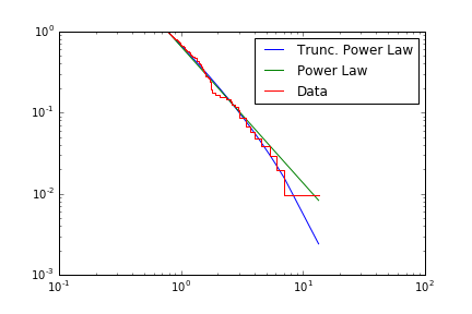
Once the distributions have been compared, the results can be plotted:

fit.truncated_power_law.plot_ccdf(label='Trunc. Power Law')
fit.power_law.plot_ccdf(label='Power Law')
fit.plot_ccdf(drawstyle='steps',label='Data')
plt.legend()