When dealing with spectral line data cubes, we will often use moments as simple descriptions of the emission in the data set. This is an aid to understanding what is happening inside the three dimensional data volume of the cube. Let’s set up a little formalism. Consider the spectral line data cube to be a map of emission on the sky, with two spatial coordinates and one spectral coordinate. Since moments only make sense when dealing with spectral line data, let us further assume that the spectral coordinate is a line-of-sight velocity calculated from the Doppler formula. Thus our cube is $I(x,y,v)$. A single spectrum at position $(x_0, y_0)$ will be denoted $T(v)$, dropping the spatial coordinate for brevity.

If we look at a spectrum of a line, it will have a form like the figure below. 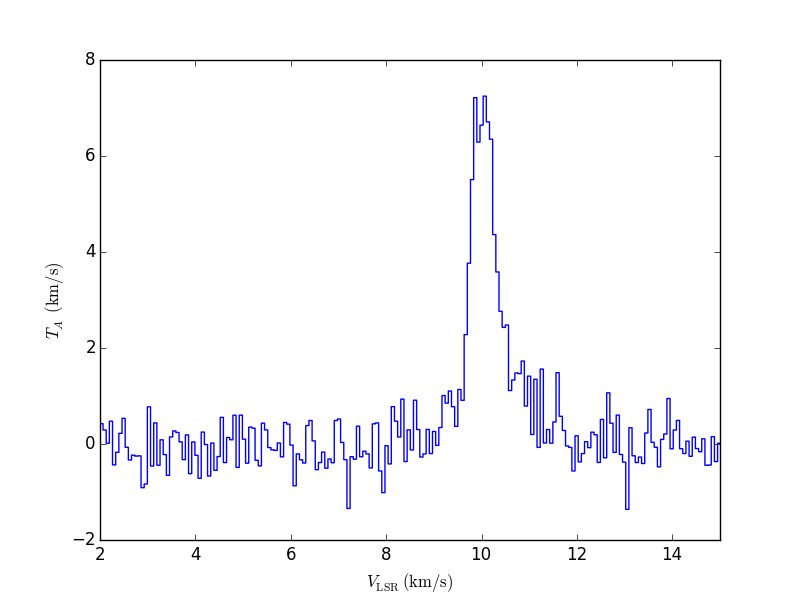The line looks roughly like a Gaussian and the “jitter” seen off the line is instrumental noise (say, around $v=4$ km/s). A compact way of describing the line would be to fit a Gaussian curve to it and simply describe the curve in terms of the three parameters of the fit, namely

$$S_{\mathrm{fit}}(v) = A \exp\left[-\frac{(v-v_0)^2}{2\sigma_v^2}\right].$$

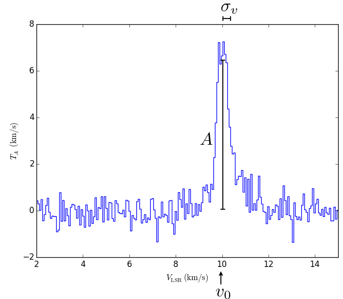
The three fit parameters are $A$, the amplitude of the line, $v_0$ which is the centre of the line, and $\sigma_0$ which is a measurements of the line width. These are annotated in the figure below. The $A$ value will have units of the $y$-axis (here Kelvin). The line centre ($v_0$) and line width ($\sigma_0$) will have the units of the $x$-axis (here km/s).
While we can fit this line, the non-linear regression of a Gaussian can be unstable and line profiles can also be messier, so we use moments as a separate, complementary approach.

The idea for moments is to use sums over the emission line to estimate the parameters. We define the zeroth moment (or the zeroth-order moment) as

$$M_0 = \int_{\mathrm{line}} T(v)\,dv \approx \sum_{i\in\{\mathrm{line}\}} T(v_i)\,\delta v.$$

This is the area under the curve, which we approximate as the sum of the spectrum over the velocity channels in the line. Velocity channels are the discrete samples in the spectrum. They each have an associated width $\delta v$ which is taken to be uniform in our applications, though analogous moments in optical data can have varying channel widths. Because we are (approximately) integrating the spectrum, $M_0$ is often called the integrated intensity.

Note that the sum over channels with the line in them is necessarily well defined. In noisy data, how can we determine where the line ends and the noise begins? There are many techniques for doing so. In the case of the integrated intensity, we don’t worry too much because the noise fluctuations should be around $T=0$ so we add roughly positive and negative contributions. This makes the estimate of $M_0$ a little noisier but should not change its value. The default behaviour is to sum over the entire spectrum, but this can be improved by masking, which means ignoring data which is likely to be only noise.

The first moment is defined as

$$M_1 = \frac{\int_{\mathrm{line}} v T(v)\,dv}{\int_{\mathrm{line}} T(v)\,dv} \approx \frac{\sum_{i\in\{\mathrm{line}\}} v_i T(v_i)\,\delta v}{M_0}.$$

This formulation should look somewhat familiar: it looks a lot like a one-dimensional centre-of-mass calculation. Indeed, the first moment is a measure of the centre-of-emission over the line. We therefore call this the velocity centroid. Note the normalization by the integrated intensity so that the resulting units of $M_1$ are in units of the line-of-sight velocity $v$. For a Gaussian line profile and no noise, $M_1= v_0$ in the spectrum figure above. We use this as an approximation, but again, the noise will cause there to be some errors in this estimator. Masking will limit this uncertainty.

The final moment we usually consider is second moment:

$$M_2 = \frac{\int_{\mathrm{line}} (v-v_0)^2 T(v)\,dv}{\int_{\mathrm{line}} T(v)\,dv} \approx \frac{\sum_{i\in\{\mathrm{line}\}} (v_i-M_1)^2 T(v_i)\,\delta v}{M_0}.$$

This is an estimate of the variance of $v$ around the line centroid $v_0$. Practically, we use the estimator $M_1$ for the line centroid. We use this estimator as a measurement of the line width, $M_2\approx \sigma_v^2$.

From here, we define higher order moments though we use them rarely:

$$M_n = \frac{\int_{\mathrm{line}} (v-v_0)^n T(v)\,dv}{\int_{\mathrm{line}} T(v)\,dv} \approx \frac{\sum_{i\in\{\mathrm{line}\}} (v_i-M_1)^n T(v_i)\,\delta v}{M_0}$$

We have special names for $M_3$ and $M_4$. We call $M_3$ the skewness since $M_3=0$ for a symmetric line profile; $M_3<0$ if the line profile has long tail for $v<v_0$; and $M_3>0$ for $v>v_0$. We define the kurtosis as $M_4-3$ since $M_4=3$ for a Gaussian line. Then the kurtosis is less than zero if the line width has narrow tails with respect to the Gaussian and is more centrally concentrated. The kurtosis is larger than zero if the line has broad tails.

You may note that we have not made an estimator of the amplitude $A$. Usually, this value is taken as the maximum of the spectrum over the line:

$$T_{\mathrm{max}} = \mathrm{max}_{i\in\{\mathrm{line}\}} T(v_i),$$

which also provides an estimate of the centroid

$$v_{\mathrm{max}} = \mathrm{argmax}_{i\in\{\mathrm{line}\}} T(v_i),$$

where $\mathrm{argmax}$ means the velocity channel at which the maximum is found (more details here.

Caveats:

• Remember that moment can be more susceptible to instrumental noise than Gaussian fits in estimating the parameters of the line.
• Masking is essential for higher order moments and dramatically improves all moments, but there is a risk that the masking will clip out real line emission, biasing the moment estimators.
• Moment estimators are defined for all line profiles, not just Gaussians. However, the values must be interpreted with care. For example, if there are two velocity components(i.e., the line is well described by a sum of two Gaussians), the velocity dispersion will represent the separation between the Gaussians.